General probabilistic theories and meta-theoretical knowledge

The vast body of scientific knowledge is a whole divided into three parts, or layers. The first falls under the name of empirical knowledge, and includes the descriptions and the results of all experiments ever attempted. The second part comprises the mathematical systematisations of those experiments and the rules to predict the outcomes of future ones, that is, the physical theories of Nature. There is also a third part, to which one may ascribe the abstract study of physical theories themselves, seen as mathematical and logical objects. The purpose of this blog post is to advocate the importance of this ‘meta-theoretical’  layer of knowledge from a conceptual and foundational standpoint, and to illustrate how it is possible to investigate it.

Meta-theoretical knowledge

If you are familiar enough with quantum information, I bet you have already heard of at least one meta-theoretical statement — a very important one. Before we come to that, let us give some examples to clarify the above tripartite categorisation of knowledge. Since this blog is about quantum mechanics, that will be our arena. In this context, our knowledge of the double-slit experiment and of its profoundly surprising results is undoubtedly empirical. Building on this and other experiments, physicists have come up with a mathematical theory of physical phenomena at the microscopic level, called quantum mechanics. Quantum mechanics, with its internal structure made of Hilbert spaces, wave functions, Born rules for measurement and collapse, and so on and so forth, is among the most luminous and successful physical theories, and thus belongs to the second layer of knowledge. One of the most striking phenomena whose existence is predicted by quantum mechanics is entanglement, i.e. the fact that distant particles may be left by previous interactions in a state that produces impossibly strong correlations upon local measurements on the two particles. The precise meaning of the words ‘impossibly strong’ was clarified by J.S. Bell in his groundbreaking 1964 paper: those correlations cannot be explained by any local hidden variable model, i.e. they are fundamentally non-local. I want to argue that this deduction — nowadays known as Bell’s theorem — is the prime example of a meta-theoretical statement. To understand why, note that Bell’s theorem has basically nothing to do with quantum mechanics; rather, it concerns its experimental predictions. It is these predictions, and not merely quantum mechanics, that are claimed to be incompatible with a local hidden variable model. In other words, any alternative theory that happened to predict the same experimental outcomes with the same probabilities (at least in the context of a Bell test) would run into the same problem, the existence of non-local correlations. Since Bell’s theorem applies to a whole class of theories, i.e. those whose experimental predictions of the outcomes of a Bell test coincide with those of quantum theory, it is a truly meta-theoretical statement. Not only: its importance lies precisely in this feature. Every person who is familiar with the formalism of quantum mechanics can see that it is intrinsically ‘non-local’, because of the way post-measurement collapses work. But this observation alone is not worth much; what if the true theory of Nature were not quantum mechanics? We cannot draw conclusions about the deepest mysteries of Nature based on our formalism; instead, we need meta-theoretical statements to certify that the bizarre phenomenon we are facing does not admit a more ‘mundane’ explanation in the context of some alternative theory.

What is a physical theory?

This discussion should convince the reader of the conceptual importance of meta-theoretical results. That being said, how do we study a set of theories that we do not even know? How do we formalise the abstract concept of a ‘physical theory’? An answer to these questions is provided by the machinery of general probabilistic theories, which we now set out to describe.

In quantum information and more generally in information theory it is common to take an operational approach to problems: a concept is defined and characterised by what allows you to do. Thus, a physical theory is for us simply a set of rules that allow to deduce a probabilistic prediction of the outcome of an experiment given the detailed description of its preparation. The above definition is quite broad. Let us discuss some of its main features. For a start, (i) ‘probabilistic’, as opposed to ‘deterministic’, refers to the fact that it is conceivable that the theory determines only the probabilities of recording the various outcomes rather than producing a definite prediction of what the outcome will be. This is the case, for instance, for quantum mechanics, which we definitely want to consider as a legitimate theory. A second observation is that (ii) the above definition depends on the set of experiments under examination; the smaller the set, the larger the number of possible theories. This is in general a desirable feature, as long as we want to be able to declare e.g. Newtonian gravity a fully-fledged physical theory, although it can only explain the motion of slow massive bodies and gets into trouble when one brings electromagnetic phenomena or relativistic speeds into the picture. A third remarkable feature of our definition of a physical theory is that (iii) it does not necessarily describe systems that evolve in time. Instead, it takes an ‘input-output’ point of view: an experiment is described as a procedure starting with a preparation of a physical system and ending with the reading of some digits on a screen. Of course, we can decide to track time evolution by designing a whole set of experiments on identically prepared systems ending at different times, but this need not be the case; depending on the context, we can content ourselves with a much more essential description of a more limited set of experiments.

Ludwig’s theorem

With this premise, we can now study the simplest physical theories of all: those that describe a single system. Such a system — that can be an atom, an electron, but also Schrödinger’s cat, depending on your stance on the issue of animal rights — can be prepared in a variety of ways, labelled by an index ω ∈ Ω, where Ω is the set of all possible preparations (hereafter called ‘states’). Also the measuring apparatus that we employ to measure the system can be set up in different ways; each 𝝀 ∈ Λ will describe a specific outcome corresponding to a particular setting of the apparatus (hereafter called ‘effect’). In this context, a theory is simply a function 𝜇 that takes as inputs a preparation ω and a measurement outcome (together with the description of the setting of the measuring apparatus) 𝜆 and outputs a probability, i.e. a real number between 0 and 1. In mathematical terms, we write 𝜇 : Ω × Λ → [0, 1].

It may be useful to pause for a second now, and describe the familiar example of quantum mechanics in this language. For the sake of simplicity, we consider a single qubit, i.e. a 2-level quantum system. The set of states Ω comprises all 2×2 density matrices and is well-known to be representable by a 3-dimensional ball — called the Bloch ball. The shape of the set of effects Λ depends on the actual measurements that are available in our laboratory. In the best-case scenario, we can assume that all so-called positive operator-valued measurements (POVM) are experimentally accessible. When this happens, effects are 2×2 matrices 𝝀 that satisfy 0 ≤ 𝝀 ≤ 1, where 1 stands for the identity matrix, and the inequalities are to be intended in the sense of positive semidefiniteness. Finally, the function 𝜇 encodes the Born rule: 𝜇(ω, 𝝀) ≔ Tr[ω 𝝀].

In the most general (non-quantum) case, the function 𝜇 as well as the sets Ω and Λ are a priori unconstrained. However, if they are to describe a physical system, it is very reasonable to postulate that they satisfy some further properties, purely on logical grounds. We formalise these properties as axioms below.

Axiom 1. The function 𝜇 separates points of Ω and Λ, namely, if some ω₁, ω₂ ∈ Ω satisfy 𝜇(ω₁, 𝜆) ≡ 𝜇(ω₂, 𝜆) for all 𝝀 ∈ Λ, then it must be ω₁ = ω₂ . Analogously, if for given 𝝀₁, 𝝀₂ ∈ Λ one has that 𝜇(ω, 𝝀₁) ≡ 𝜇(ω, 𝝀₂) for all ω ∈ Ω, then 𝝀₁ = 𝝀₂ .

In other words: if two states can not be distinguished by any effect, then to all intents and purposes they are the same state. Analogously for the effects. This assumption is not really fundamental. On the contrary, given any pair of sets Ω and Λ and a function 𝜇 that does not satisfy Axiom 1, we can always define two modified sets Ω’ and Λ’ by identifying the elements that are not separated by 𝜇. The resulting quotient function 𝜇’ then satisfies Axiom 1  on Ω’ and Λ’ by construction.

Axiom 2. There is a ‘trivial effect’ u such that 𝜇(ω, u) ≡ 1 for all ω ∈ Ω. Moreover, for all 𝜆 ∈ Λ there is an ‘opposite effect’ 𝜆’ such that 𝜇(ω, 𝜆’) ≡ 1 − 𝜇(ω, 𝜆) for all ω ∈ Ω .

This axiom is also very natural. The trivial effect can simply be obtained by preparing the measurement apparatus to produce a fixed output. Given an effect 𝜆, setting up the apparatus exactly as described by 𝜆 and accepting all outcomes that do not correspond to 𝜆 yields its logical negation 𝜆’.

Axiom 3. Probabilistic mixtures of states (respectively, effects) are again valid states (respectively, effects). That is, for all states ω₁, ω₂ ∈ Ω and probabilities p ∈ [0,1], there exists a state 𝜏 such that 𝜇(𝜏, 𝜆) = p 𝜇(ω₁, 𝜆) + (1 – p) 𝜇(ω₂, 𝜆) for all 𝜆 ∈ Λ. Same for the effects.

What Axiom 3 is telling us is that given two preparation procedures ω₁, ω₂, it should be possible to construct their probabilistic combination. This is a third preparation procedure     𝜏 obtained by flipping a (biased or unbiased) coin, preparing the state according to ω₁ or ω₂ depending on the outcome, and then forgetting that same outcome. Clearly, 𝜏 must reproduce probabilistically the behaviour of ω₁ and ω₂ when tested on all effects 𝜆.

The formalism we have developed so far seems to be rather inconvenient, especially when compared with the quantum mechanical example described above. Let us identify its main weaknesses. (a) In quantum theory, states and effects are represented by objects in a linear vector space; this means e.g. that the state 𝜏 of Axiom 3 is simply given by the convex combination p ω₁ + (1 – p) ω₂ , which eliminates the need to go through the function 𝜇 to determine it. (b) The quantum Born rule 𝜇(ω, 𝝀) = Tr[ω 𝜆] is bilinear in the state and the effect (meaning that it is linear in each argument when the other is kept fixed). This is a very convenient property especially when long computations are involved.

To fix these inconvenient features of the 𝜇-formalism, a theorem by the German physicist Günther Ludwig comes to our rescue. It states that whenever Axioms 1,2,3 are satisfied, the sets Ω and Λ can be thought of as convex sets in linear vector spaces, so that (a) probabilistic mixtures become convex combinations; and (b) the 𝜇 function (generalised Born rule) is bilinear in the state and the effect. For completeness, we state the theorem formally below.

Theorem (Ludwig’s embedding theorem). If Axioms 1,2,3 are satisfied, there is a vector space V such that:

• Ω ⊆ V, Λ ⊆ V^* are convex sets, with 0,u ∈ Λ, and Λ = u − Λ;
• ℝ₊∙Ω = C is a cone, ℝ₊∙Λ = C^* ≔ { 𝜑 ∈ V^*:  𝜑(x) ≥ 0  ∀ x ∈ C } ⊆ V^* is the corresponding dual cone; the set of states satisfies Ω = {x ∈ C : u(x) = 1};
• the generalised Born rule holds: 𝜇(ω, 𝝀) = 𝝀(ω).

Here, the symbol V^* represents the dual of the vector space V, i.e. the space of all linear functionals acting on V. Hereafter, we shall refer to C as the cone of unnormalised states, and to the functional u as the order unit. The dual cone C^* lives in the dual space, and can be simply thought of as formed by all linear functionals that are positive on the whole C.

Note. For the sake of readability, we stated the theorem in the simple case where V is finite-dimensional. It should be noted, however, that one of the big conceptual contributions by Ludwig was to formulate and prove an embedding theorem that covers also the infinite-dimensional case, and is (unsurprisingly) much more technically involved.

Ludwig’s embedding theorem provides an elegant solution to the main problems of the 𝜇-formalism as discussed above. It is so important because it provides the foundation for the formalism of general probabilistic theories (GPTs). The theorem was proved long ago, in a series of works published between the 1960s and 1970s. Nowadays, it is implicitly used in practically any paper on GPTs. It is indeed common to start any analysis by simply assuming that the state space is a convex set in a real vector space, and that the effects are linear functionals with values between 0 and 1 on said state space. That this assumption causes no loss of generality is precisely the take-home message of Ludwig’s theorem.

The formalism of general probabilistic theories

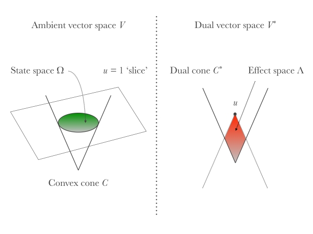
We conclude this post by summarising the formalism of GPTs as it emerges from Ludwig’s theorem (and adding the last bits and pieces). It is useful to start with a picture.

1. The cone formed by unnormalised states (positive multiples of physical states) is a proper cone C in a real vector space V . Here, ‘proper’ means that it is closed, convex, that it spans the whole space (we want to exclude the ‘flat’ case), and that it does not contain any straight line (opening angle less than 𝜋).

2. The order unit u belongs to the interior of the dual cone C^*, in turn defined as C^* = {𝜑 ∈ V^*: 𝜑(x) ≥ 0 ∀x ∈ C} ⊆ V^*;

3. The state space is obtained by slicing C with u at height 1, in formulae    Ω = {x∈ C : u(x) = 1}. Statistical mixtures of states are represented mathematically by convex combinations.

4. Measurements are represented by (finite) collections of effects ( e_i )_i∈I ⊆ Λ that add up to the order unit, i.e. such that Σ_i∈I e_i = u. The probability of obtaining the outcome i when measuring the state ω is given by the generalised Born rule: p(i|ω) = e_i (ω).

In stating (4) we made the implicit assumption that all linear functionals that take on values between 0 and 1 on Ω are legitimate effects. This assumption is commonly known as the ‘no-restriction hypothesis’, and corresponds geometrically to requiring that the effects Λ cover the whole red set on the right side of the above figure. This is not necessarily the case in many conceivable situations. For example, it may happen that our experimental apparatus is subjected to some intrinsic noise that makes sharp measurements impossible. The main justification of the no-restriction hypothesis, beyond its mathematical simplicity and elegance, lies in the fact that it is well-verified at a fundamental level in classical and quantum theory. That is, we believe it possible, at least in principle, to construct a close-to-ideal measurement apparatus that can implement any given sharp quantum measurement. Unless otherwise specified, we will always make the no-restriction hypothesis from now on.

We conclude this post by discussing some examples of GPTs.

• Classical probability theory. The system is simply a ball hidden somewhere in one out of d boxes. States represent our partial knowledge of the ball’s position, and are thus modelled by probability distributions over a discrete set of size d. The host vector space V = ℝ^d comprises all real vectors of length d, and unnormalised states form the cone ℝ₊^d of vectors with non-negative components. The order unit is the functional acting as u(x) = x₁ +…+ x_d , so that the slice u = 1 of the cone ℝ₊^d truly identifies the state space Ω as the set of all probability distributions. Its geometrical shape is that of a simplex, more precisely, a regular (d-1)-simplex. To picture a simplex in your mind, note that a regular 1-simplex is a segment, a regular 2-simplex an equilateral triangle, a regular 3-simplex a Platonic tetrahedron, and so on.

• Quantum mechanics. We discussed this important example before in the simple case of a qubit. In the quantum mechanical theory of an n-level system, the host vector space comprises all n × n Hermitian matrices. Although some of their entries may be complex, Hermitian matrices form a real vector space, closed under real (not under complex!) linear combinations. The cone C of unnormalised states is formed by all positive semidefinite matrices, and it is sliced at height 1 by the order unit functional u(X) = Tr[X] (the trace). The resulting section is the set of all n × n density matrices, i.e. positive semidefinite matrices of unit trace; we thus get back the familiar quantum formalism.

• Spherical model. As already mentioned, the state space of a single qubit is geometrically representable as a ball — the Bloch ball. This is really a peculiar feature of dimension 2, the set of quantum density matrices in higher dimension possessing a more complicated structure. However, we can take inspiration from this considerations to design a GPT whose state space is defined to be a d-dimensional ball. The way to obtain this in the GPT formalism is very easy, and is already pictorially represented in the above figure. We can take as host vector space V = ℝ^d+1 (all real vectors of length d+1), and as C the ‘ice cream cone’ formed by all vectors x = (x₀, …, x_d) such that x₀ ≥ (x₁² +…+ x_d² )^1/2 . Then, the functional u(x) = x₀ does the job of slicing C so as to produce a d-dimensional Euclidean ball.

• Generalised bit. Now that we have in our toolkit a GPT whose state space is a Euclidean ball, why not construct one whose state space has a cubical shape? More precisely, we want Ω to be the d-dimensional hypercube, which can be mathematically defined as the convex hull of all points in ℝ^d with coordinates ±1. This is more easily done that said. Let the ambient vector space be V = ℝ^d+1 (as before), and take C as the cone formed by all vectors x = (x₀, …, x_d) such that x₀ ≥ max{x₁ ,…, x_d }. It is not difficult to verify that the same order unit functional u(x) = x₀ determines on C a section shaped as a d-dimensional hypercube.

This concludes our introduction to the modern formalism of general probabilistic theories. We have seen how this emerges naturally from a very broad definition of the notion of physical theory via Ludwig’s theorem, and we discussed a few (hopefully instructive) examples. For those who would like to know more about the early days of the GPT formalism, and especially delve into some of the mathematical details, I warmly recommend having a look at [1]. The original proof of Ludwig’s theorem can be found in [2] and references therein. I tried to give a self-contained account of it with all the technical details in Chapter 1 of my PhD thesis [3]. Chapter 2 of the same thesis summarises instead the GPT formalism in finite dimension.

[1] A. Hartkämper and H. Neumann. Foundations of Quantum Mechanics and Ordered Linear Spaces: Advanced Study Institute held in Marburg 1973. Springer Berlin Heidelberg, 1974.

[2] G. Ludwig. An Axiomatic Basis for Quantum Mechanics: Derivation of Hilbert space structure, volume 1. Springer-Verlag, 1985.

[3] L. Lami. Non-classical correlations in quantum mechanics and beyond. PhD thesis, Universitat Autònoma de Barcelona, October 2017. Preprint arXiv:1803.02902.